Convolution层的实现---以caffe为例

Mar.11-2017

前段时间尝试去重现了下卷积层的具体实现，网上看了些blog，但是发现的现状是好多文章都是相互抄袭，到最后自己都不知道讲什么。于是自己详细梳理了下卷积层的具体实现，并以caffe为例详细了解下代码实现。

卷积层的基本原理与加速

我们知道从filter的角度来看待Convolution层，其实就是我们用不同的filter来对输入层做卷积生成一个输出。具体来说如下图：
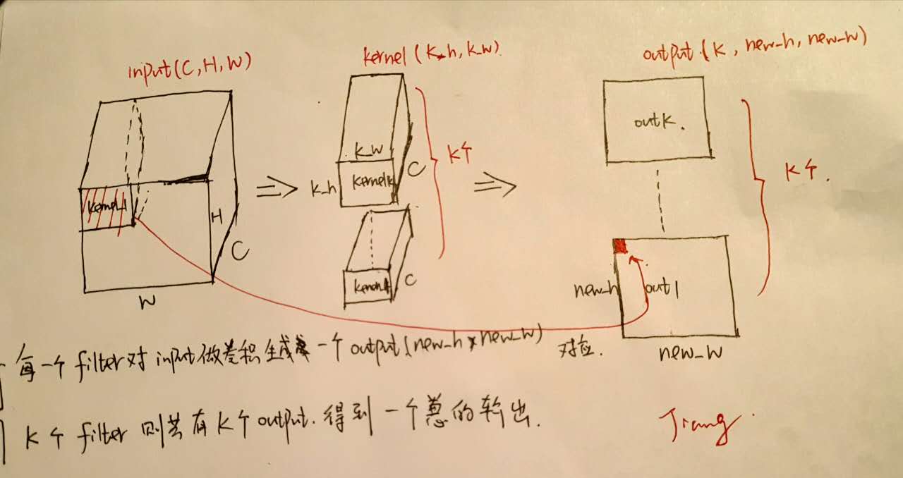conv 假设Input的大小为$(C, H, W)$，其中$C$为channel数，$H$为高度，$W$为宽度。

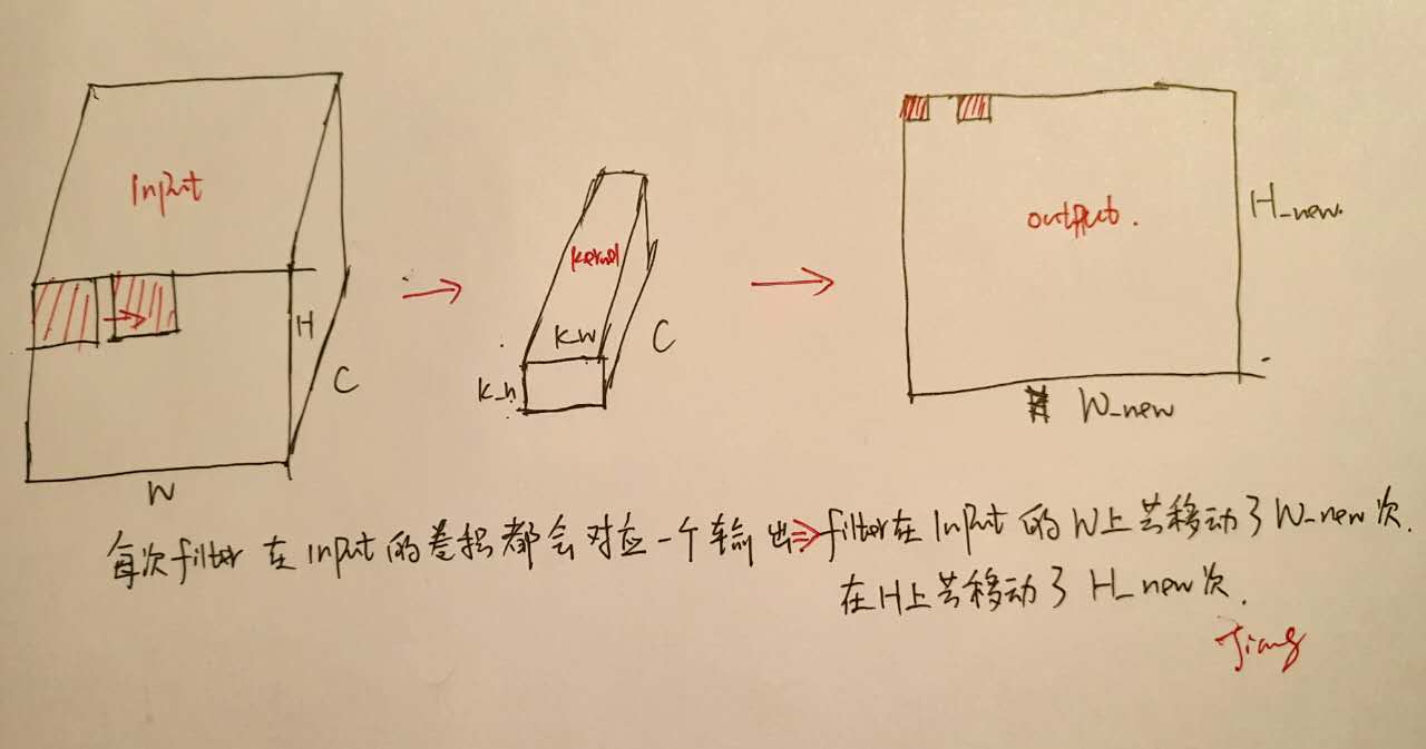
定义filter的大小为$(F_h, F_w)$，那么filter的channel数是默认为$C$的。并且定义$pad$的大小为$P$, $stride$的大小为$S$。

那么output的得到过程是这样的，我们将filter放在左上方初始的位置，然后每次以$stride$大小进行移动，每次将filter与Input对应的部分进行卷积，得到一个output输出点—如上图所示每个output都与一个Input区域一一对应，这样我们便生成了一个feature_map，将$K$个filter的结果结合起来我们便得到了一个输出$K, H_{new}, W_{new}$。并且我们可以根据上述过程推导得到output的大小：
$H_{new} = \frac{H + 2P - F}{S} + 1$
$W_{new} = \frac{W + 2P - F}{S} + 1$
有兴趣的朋友可以自己去推导一下，一个更形象的filter过程可以参考cs231n中的一个例子，如下所示：

那么当我们想要计算输出的时候只需要模拟上述过程不断地用filter去输入上进行卷积即可得到输出。
但是我们不要忘了所谓的卷积只是矩阵乘法而已，能不能进行加速呢？答案是可以的！如下以一个filter为例子所示：
filter 上图解释了output的生成过程，注意到output上的每一个点都对应于Input上不同的位置与相同的filter做矩阵乘法的结果—这就是我们加速的关键之处—将所有的可能Input位置一次性找出来，然后与filter做矩阵乘法，一步得到output输出！而K个filter的情况不过是一个拓展而已。

具体的一个例子：
如果我们的Input大小为$(3, 227, 227)$，我们以一个$(3, 11, 11)$的filter对其进行卷积，$stride$大小为4。我们将每次与filter进行计算的输入区域展开为一个列向量，那么其大小为$3 \times 11 \times 11 = 363$，在Input上共有$H_{new} = \frac{227 - 11}{4} + 1 = 55, W_{new} = \frac{227 - 11}{4} + 1 = 55$个参加计算的位置，一共$55 \times 55 = 3025$将这些列向量进行拼接我们便得到了一个矩阵$x_{col}$，其大小为$[363 \times \ 3025]$，这一过程叫做im2col

同时我们将每一个filter展开为一个行向量，大小为$363$，假设我们共有$K$个filter，那么我们得到另一个矩阵$W_{row}$，大小为$[K \times 363]$

将这两个矩阵相乘$W_{row} \times x_{col}$，得到output，大小为$[K \times 3025]$,再resize回去即可得到我们的输出。

可以看到我们只进行了一次矩阵的乘法便得到了输出，唯一的缺点在于由于$x_{col}$中有大量的重复数据，我们会占用更多的内存。但是$x_{col}$的引入除了加速外也使得前向反向传播变得很清晰。

考虑从上一层反向传播过来的$diff = \frac{\partial Loss}{\partial output}$,当我们要进行反向传播和参数更新时十分直观:
$\frac{\partial Loss}{\partial W_{row}} = diff \times \frac{\partial out}{\partial W_{row}} = diff \times x_{col} （1）$
对于反向传播因为前向传播时只有$x_{col}$参与其中，那么反向传播时也只有这些数据会被传播到，所以 $\frac{\partial Loss}{\partial input} = diff \times \frac{\partial out}{\partial x_{col}} = diff \times W_{row} （2）$

可以看到$x_{col}$的引入是十分有利的，而这也是现在大多数深度学习框架对Convolution层的具体实现方式，下面以caffe为例子，从代码层面进行具体的阐述。

caffe中的卷积层实现

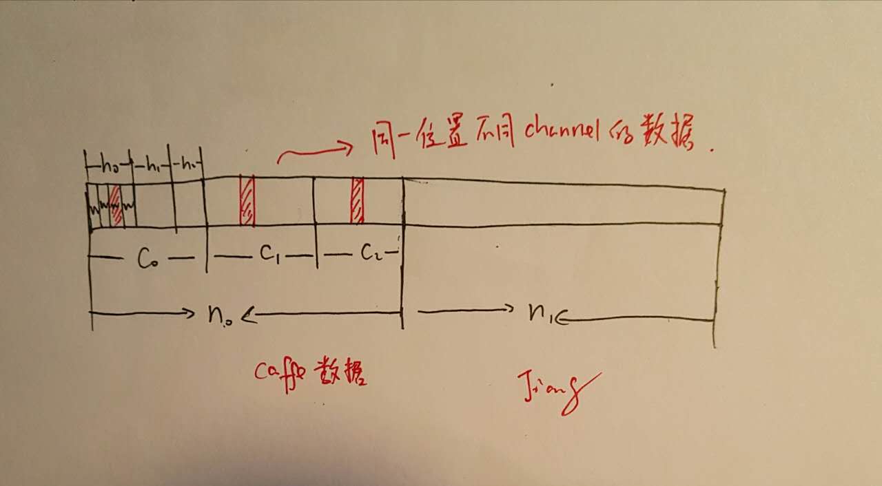
在具体讲解代码以前我们需要先对caffe的数据存储进行一下了解，caffe中数据都是通过blob来进行存储传播的，blob是对于底层数据的一个封装，其数据存储的顺序为$(N,C,H,W)$，当然实际上是存储为一维数组的，对于一个$(n, c, h, w)$的数据点来说其具体位置是:$(n \times C + h) \times H + w$,如下所示存储结构:
blob 同时回忆一下$x_{col}$和$w_{row}$的具体内容:
$x_{col} = (C \times H_{kernel} \times W_{kernel}) \times (H_{new} \times W_{new})$
$w_{row} = K \times (C \times H_{kernel} \times W_{kernel})$

了解了数据存储方式，下面我们来具体看caffe中的具体实现，前向传播的代码存在于forward方法中，而反向传播存在于backward方法中。查看forward中的关键代码，其中调用了基类的函数

this->forward_cpu_gemm(bottom_data + n * this->bottom_dim_, weight,
          top_data + n * this->top_dim_);

下面我们来详细看一下这个函数

template <typename Dtype>
void BaseConvolutionLayer<Dtype>::forward_cpu_gemm(const Dtype* input,
    const Dtype* weights, Dtype* output, bool skip_im2col) {
  const Dtype* col_buff = input;
  if (!is_1x1_) {
    if (!skip_im2col) {
    // 此处为关键---im_col的生成
      conv_im2col_cpu(input, col_buffer_.mutable_cpu_data()); 
    }
    col_buff = col_buffer_.cpu_data();
  }
  // 下面为im_col与w_row的矩阵相乘
  for (int g = 0; g < group_; ++g) {
    caffe_cpu_gemm<Dtype>(CblasNoTrans, CblasNoTrans, conv_out_channels_ /
        group_, conv_out_spatial_dim_, kernel_dim_,
        (Dtype)1., weights + weight_offset_ * g, col_buff + col_offset_ * g,
        (Dtype)0., output + output_offset_ * g);
  }
}

我们先来说一下conv_im2col_cpu这个函数，它是整个conv层的关键，即将原始的Input转换为$x_{col}$，下面在代码层里予以详细说明整个生成过程

template <typename Dtype>
void im2col_cpu(const Dtype* data_im, const int channels,
    const int height, const int width, const int kernel_h, const int kernel_w,
    const int pad_h, const int pad_w,
    const int stride_h, const int stride_w,
    const int dilation_h, const int dilation_w,
    Dtype* data_col) {
    //计算H_new以及W_new，根据公式(H + 2P - F) / S + 1
    //这里的dilation_h为对kernel的一个缩放，可以略过
  const int output_h = (height + 2 * pad_h -
    (dilation_h * (kernel_h - 1) + 1)) / stride_h + 1;
  const int output_w = (width + 2 * pad_w -
    (dilation_w * (kernel_w - 1) + 1)) / stride_w + 1;
    // 这里channel_size可以结合前面caffe中的数据存储来看，每个channel都有
    // height * width那么多数据
  const int channel_size = height * width;
  /**
  // 下面是具体的实现过程了，回忆x_col的结构以及caffe的存储结构
  // 我们要生成的是以(C * kernel_h * kernel_w)为列，(H_new * W_new)为行的矩阵
  //但是注意这在caffe中都是一维的，每一行其实是kernel中的一个点对原图进行采样
  // 卷积的过程，下面会接着用图进行讲解
  // 前三个for为C,kernel-h,kernel_w它们控制了一共有多少行（一列）
  **/
  for (int channel = channels; channel--; data_im += channel_size) {
    for (int kernel_row = 0; kernel_row < kernel_h; kernel_row++) {
      for (int kernel_col = 0; kernel_col < kernel_w; kernel_col++) {
      
      // 下面是对于每一行的数据生成过程
      // 对于一行，找到kernel中的对应点开始进行在input中进行卷积的h的初始位置
        int input_row = -pad_h + kernel_row * dilation_h;
        for (int output_rows = output_h; output_rows; output_rows--) {
        // 如果目前的位置h是小于0或者大于Input_h的，那么对该输出行填充0
          if (!is_a_ge_zero_and_a_lt_b(input_row, height)) {
            for (int output_cols = output_w; output_cols; output_cols--) {
              *(data_col++) = 0;
            } // 对一个output_w填充0
          } else {
          // 如果目前h不是0，那么找到初始的w开始的位置，开始进行这一行的填充
            int input_col = -pad_w + kernel_col * dilation_w;
            for (int output_col = output_w; output_col; output_col--) {
            // 判断现在这一位置是不是小于0或者大于width，不是则填充数据否则为0
              if (is_a_ge_zero_and_a_lt_b(input_col, width)) {
                *(data_col++) = data_im[input_row * width + input_col];
              } else {
                *(data_col++) = 0;
              }
              // w横向位置的递增
              input_col += stride_w;
            } // 对一个output_w的填充完成
          }
          // h纵向位置的递增，转移到下一个output_w
          input_row += stride_h;
        }// 完成整个x_col一行的数据填充，为output_h * output_w
        
      }
    }
  }
}

下面结合下图来对上述代码中的注解进行进一步阐述。 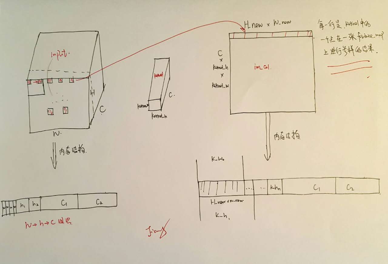x_col 按照caffe的存储结构,在实际生成$x_{col}$的每一行的时候，其实是模拟kernel中的一个点在feature_map上的一层进行采样，然后不停地更新该点以及更新feature_map得到最终结果(for循环的前三层)
在反向传播的过程又是怎样的呢？照例看看代码的关键部分

// 更新weight
this->weight_cpu_gemm(bottom_data + n * this->bottom_dim_,
              top_diff + n * this->top_dim_, weight_diff);
 // 反向传播             
this->backward_cpu_gemm(top_diff + n * this->top_dim_, weight,
              bottom_diff + n * this->bottom_dim_);

详细看这两个函数的代码

template <typename Dtype>
void BaseConvolutionLayer<Dtype>::weight_cpu_gemm(const Dtype* input,
    const Dtype* output, Dtype* weights) {
  const Dtype* col_buff = input;
  if (!is_1x1_) {
  // 计算im_col
    conv_im2col_cpu(input, col_buffer_.mutable_cpu_data());
    col_buff = col_buffer_.cpu_data();
  }
  for (int g = 0; g < group_; ++g) {
  // 与(1)一致，该层gradient等于diff乘以x_col
    caffe_cpu_gemm<Dtype>(CblasNoTrans, CblasTrans, conv_out_channels_ / group_,
        kernel_dim_, conv_out_spatial_dim_,
        (Dtype)1., output + output_offset_ * g, col_buff + col_offset_ * g,
        (Dtype)1., weights + weight_offset_ * g);
  }
}

可以看到参数的更新与我们分析的一致，符合(1)式。

template <typename Dtype>
void BaseConvolutionLayer<Dtype>::backward_cpu_gemm(const Dtype* output,
    const Dtype* weights, Dtype* input) {
    // 得到col_buff数据
  Dtype* col_buff = col_buffer_.mutable_cpu_data();
  if (is_1x1_) {
    col_buff = input;
  }
  for (int g = 0; g < group_; ++g) {
  // 反向传播，与(2)式一致
    caffe_cpu_gemm<Dtype>(CblasTrans, CblasNoTrans, kernel_dim_,
        conv_out_spatial_dim_, conv_out_channels_ / group_,
        (Dtype)1., weights + weight_offset_ * g, output + output_offset_ * g,
        (Dtype)0., col_buff + col_offset_ * g);
  }
  if (!is_1x1_) {
    conv_col2im_cpu(col_buff, input);
  }
}

反向传播的过程也与分析(2)一致，diff乘以weight，只有x_col对应的部分得到了反向传播的影响。

小结

至此convolution层的基本实现加速就分析完了，可以看到将原来的分批卷积操作转换为矩阵的乘法，不仅可以加速计算还可以使得参数的更新以及反向传播变得清洗明了，在内存允许的情况下是个不错的实现手段。